sample_arc_from_normal()

Sample mesh data along a circular arc defined by a normal vector.

Creates a circular arc probe defined by a normal to the plane of the arc, a polar starting vector, and an angle. The arc is sampled in a counterclockwise direction from the polar vector. For temporal datasets, automatically sweeps all time points unless time_value is specified.

Parameters

• center (Sequence[float]) — Center point [x, y, z] of the circle that defines the arc.
• resolution (int, default: 100) — Number of segments to divide the arc into. The resulting arc will have resolution + 1 points.
• normal (Sequence[float] | None, default: None) — Normal vector [x, y, z] to the plane of the arc. If None, defaults to [0, 0, 1] (positive Z direction).
• polar (Sequence[float] | None, default: None) — Starting point of the arc in polar coordinates [x, y, z]. If None, defaults to [1, 0, 0] (positive X direction).
• angle (float | None, default: None) — Arc length in degrees, beginning at the polar vector in a counterclockwise direction. If None, defaults to 90 degrees.
• time_value (float | None, default: None) — Query a specific time value instead of sweeping all time points. Ignored for static datasets.
• tolerance (float | None, default: None) — Tolerance for the sample operation. If None, PyVista generates a tolerance automatically.

Returns

Returns a list of dictionaries (one per time step) with a "time" key and array names as keys. Each array has:

• For scalars: "distance", "value", "x", "y", "z" (sample point coordinates)
• For vectors: "distance", "x_value", "y_value", "z_value", "tangential" (component along arc), "normal" (component perpendicular to arc), "x", "y", "z" (sample point coordinates)

For static datasets, returns a single-element list with time 0.0.

[
    # Time 0 (or single time for static)
    {
        "time": 0.0,
        "scalar_name": {
            "distance": [0.0, 0.1, 0.2, ...],
            "value": [val0, val1, val2, ...],
            "x": [x0, x1, x2, ...],
            "y": [y0, y1, y2, ...],
            "z": [z0, z1, z2, ...]
        },
        "vector_name": {
            "distance": [0.0, 0.1, 0.2, ...],
            "x_value": [x0, x1, x2, ...],
            "y_value": [y0, y1, y2, ...],
            "z_value": [z0, z1, z2, ...],
            "tangential": [t0, t1, t2, ...],
            "normal": [n0, n1, n2, ...],
            "x": [x0, x1, x2, ...],
            "y": [y0, y1, y2, ...],
            "z": [z0, z1, z2, ...]
        },
        ...
    },
    # Time 1
    {"time": 0.01, ...},
    ...
]

Examples

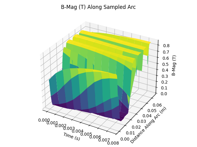
Sweep all time steps

from pyemsi import Plotter, examples
from matplotlib import pyplot
import numpy as np

file_path = examples.ipm_motor_path()
plt = Plotter(file_path)

data = plt.sample_arc_from_normal(
    center=(0, 0, 0),
    normal=(0, 0, 1),
    polar=(0.080575, 0, 0),
    angle=45,
    resolution=100,
)

time_values = [time_data["time"] for time_data in data]
distances = data[0]["B-Mag (T)"]["distance"]
value_grid = np.array([time_data["B-Mag (T)"]["value"] for time_data in data])
time_grid, distance_grid = np.meshgrid(time_values, distances, indexing="ij")

fig, ax = pyplot.subplots(subplot_kw={"projection": "3d"})
ax.plot_surface(time_grid, distance_grid, value_grid, cmap="viridis")
ax.set_xlabel("Time (s)")
ax.set_ylabel("Distance Along Arc (m)")
ax.set_zlabel("B-Mag (T)")
ax.set_title("B-Mag (T) Along Sampled Arc")
fig.tight_layout()
fig.savefig("docs/static/demos/sample_arc_from_normal.png")

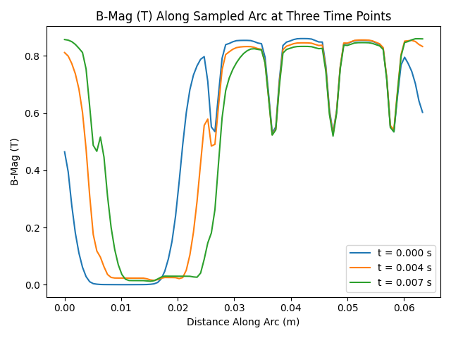
Plot three time slices

from pyemsi import Plotter, examples
from matplotlib import pyplot

file_path = examples.ipm_motor_path()
plt = Plotter(file_path)

data = plt.sample_arc_from_normal(
    center=(0, 0, 0),
    normal=(0, 0, 1),
    polar=(0.080575, 0, 0),
    angle=45,
    resolution=100,
)
time_indices = sorted({0, len(data) // 2, len(data) - 1})

fig, ax = pyplot.subplots()
for idx in time_indices:
    ax.plot(
        data[idx]["B-Mag (T)"]["distance"],
        data[idx]["B-Mag (T)"]["value"],
        label=f"t = {data[idx]['time']:.3f} s",
    )
ax.set_xlabel("Distance Along Arc (m)")
ax.set_ylabel("B-Mag (T)")
ax.set_title("B-Mag (T) Along Sampled Arc at Three Time Points")
ax.legend()
fig.tight_layout()
fig.savefig("docs/static/demos/sample_arc_from_normal_time_slices.png")

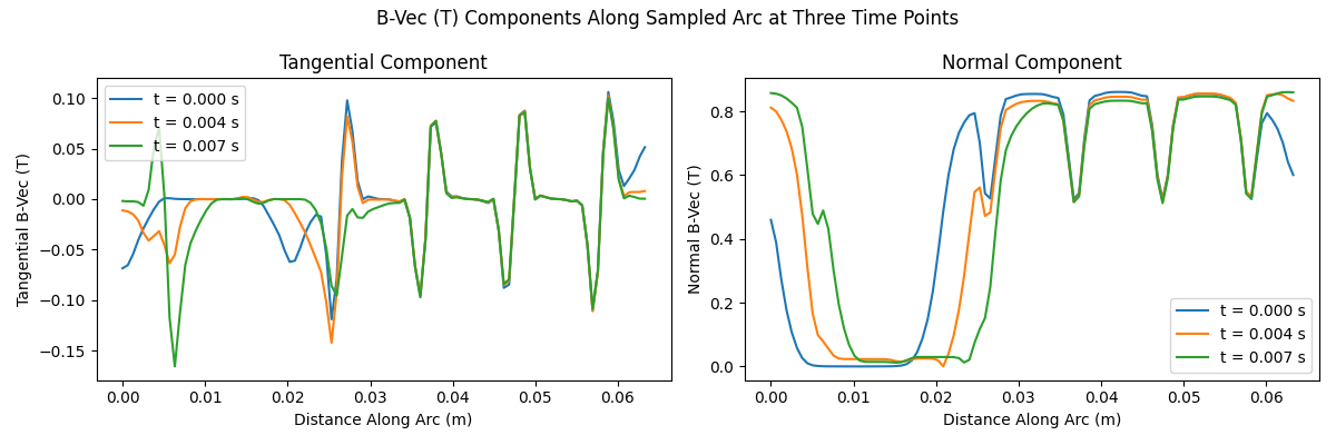
Plot tangential and normal B-Vec components

from pyemsi import Plotter, examples
from matplotlib import pyplot
import numpy as np

file_path = examples.ipm_motor_path()
plt = Plotter(file_path)

data = plt.sample_arc_from_normal(
    center=(0, 0, 0),
    normal=(0, 0, 1),
    polar=(0.080575, 0, 0),
    angle=45,
    resolution=100,
)
time_indices = sorted({0, len(data) // 2, len(data) - 1})

fig, axes = pyplot.subplots(1, 2, figsize=(12, 4))
component_map = [
    ("tangential", "Tangential B-Vec (T)"),
    ("normal", "Normal B-Vec (T)"),
]

for ax, (component_key, ylabel) in zip(np.atleast_1d(axes), component_map):
    for idx in time_indices:
        ax.plot(
            data[idx]["B-Vec (T)"]["distance"],
            data[idx]["B-Vec (T)"][component_key],
            label=f"t = {data[idx]['time']:.3f} s",
        )

    ax.set_xlabel("Distance Along Arc (m)")
    ax.set_ylabel(ylabel)
    ax.legend()

axes[0].set_title("Tangential Component")
axes[1].set_title("Normal Component")
fig.suptitle("B-Vec (T) Components Along Sampled Arc at Three Time Points")
fig.tight_layout()
fig.savefig("docs/static/demos/sample_arc_from_normal_bvec_components_time_slices.png")

Notes

• The arc is constructed in a counterclockwise direction from the polar vector as viewed from the direction of the normal vector.
• The default normal [0, 0, 1] and polar [1, 0, 0] create an arc in the XY plane starting from the positive X axis.
• For vectors, tangential represents the component along the arc direction, while normal represents the magnitude perpendicular to the arc.
• The "x", "y", "z" keys contain the actual 3D coordinates of sample points along the arc.
• This method is useful when you want to define an arc by plane orientation rather than explicit start/end points.

See Also

• sample_arc() - Sample along arc defined by start/end points
• sample_arcs_from_normal() - Sample multiple arcs defined by normal vectors
• sample_line() - Sample along straight line