sample_arcs()
Sample mesh data along multiple circular arcs.
Creates circular arc probes for each (pointa, pointb, center) tuple and samples the mesh data onto each arc. For temporal datasets, automatically sweeps all time points unless time_value is specified.
Parameters
arcs(Sequence[tuple[Sequence[float], Sequence[float], Sequence[float]]]) — List of arc definitions, each as a tuple(pointa, pointb, center)where each component is an[x, y, z]coordinate.resolution(int | list[int], default:100) — Number of segments to divide each arc into. Can be a singleint(applied to all arcs) or a list ofints (one per arc).negative(bool, default:False) — IfFalse, arcs span the positive angle. IfTrue, span the negative (reflex) angle. Applied to all arcs.time_value(float | None, default:None) — Query a specific time value instead of sweeping all time points. Ignored for static datasets.tolerance(float | None, default:None) — Tolerance for the sample operation. IfNone, PyVista generates a tolerance automatically.progress_callback(callable | None, default:None) — Callback function for progress updates. Called with(current_arc, total_arcs). Should returnTrueto continue orFalseto cancel.
Returns
Returns a list of results (one per arc), where each result is a list of dictionaries (one per time step) with a "time" key and array names as keys. Each array has:
- For scalars:
"distance","value","x","y","z"(sample point coordinates) - For vectors:
"distance","x_value","y_value","z_value","tangential","normal","x","y","z"(sample point coordinates)
[
    # First arc results
    [
        # Time 0
        {"time": 0.0, "scalar_name": {"distance": [...], "value": [...], "x": [...], "y": [...], "z": [...]}, ...},
        # Time 1
        {"time": 0.01, "scalar_name": {"distance": [...], "value": [...], "x": [...], "y": [...], "z": [...]}, ...},
        ...
    ],
    # Second arc results
    [
        {"time": 0.0, "scalar_name": {"distance": [...], "value": [...], "x": [...], "y": [...], "z": [...]}, ...},
        ...
    ],
    ...
]
Examples
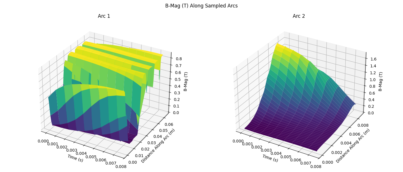
Sweep all time steps
from pyemsi import Plotter, examples
from matplotlib import pyplot
import numpy as np

file_path = examples.ipm_motor_path()
plt = Plotter(file_path)

data = plt.sample_arcs(
    arcs=[
        ((0.080575, 0, 0), (0.0569751, 0.0569751, 0), (0, 0, 0)),
        ((0.0792007, 0.0167379, 0), (0.0769587, 0.0251049, 0), (0, 0, 0)),
    ],
    resolution=100,
)

fig, axes = pyplot.subplots(1, len(data), figsize=(14, 6), subplot_kw={"projection": "3d"})
axes = np.atleast_1d(axes)

for idx, arc_data in enumerate(data):
    time_values = [time_data["time"] for time_data in arc_data]
    distances = arc_data[0]["B-Mag (T)"]["distance"]
    value_grid = np.array([time_data["B-Mag (T)"]["value"] for time_data in arc_data])
    time_grid, distance_grid = np.meshgrid(time_values, distances, indexing="ij")

    axes[idx].plot_surface(time_grid, distance_grid, value_grid, cmap="viridis")
    axes[idx].set_xlabel("Time (s)")
    axes[idx].set_ylabel("Distance Along Arc (m)")
    axes[idx].set_zlabel("B-Mag (T)")
    axes[idx].set_title(f"Arc {idx + 1}")

fig.suptitle("B-Mag (T) Along Sampled Arcs")
fig.tight_layout()
fig.savefig("docs/static/demos/sample_arcs.png")
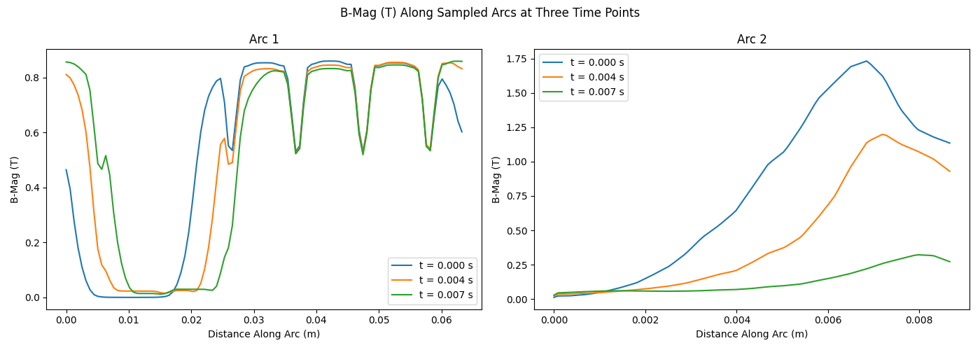
Plot three time slices
from pyemsi import Plotter, examples
from matplotlib import pyplot
import numpy as np

file_path = examples.ipm_motor_path()
plt = Plotter(file_path)

data = plt.sample_arcs(
    arcs=[
        ((0.080575, 0, 0), (0.0569751, 0.0569751, 0), (0, 0, 0)),
        ((0.0792007, 0.0167379, 0), (0.0769587, 0.0251049, 0), (0, 0, 0)),
    ],
    resolution=100,
)

fig, axes = pyplot.subplots(1, len(data), figsize=(14, 5))
axes = np.atleast_1d(axes)

for idx, arc_data in enumerate(data):
    time_indices = sorted({0, len(arc_data) // 2, len(arc_data) - 1})

    for time_idx in time_indices:
        axes[idx].plot(
            arc_data[time_idx]["B-Mag (T)"]["distance"],
            arc_data[time_idx]["B-Mag (T)"]["value"],
            label=f"t = {arc_data[time_idx]['time']:.3f} s",
        )

    axes[idx].set_xlabel("Distance Along Arc (m)")
    axes[idx].set_ylabel("B-Mag (T)")
    axes[idx].set_title(f"Arc {idx + 1}")
    axes[idx].legend()

fig.suptitle("B-Mag (T) Along Sampled Arcs at Three Time Points")
fig.tight_layout()
fig.savefig("docs/static/demos/sample_arcs_time_slices.png")
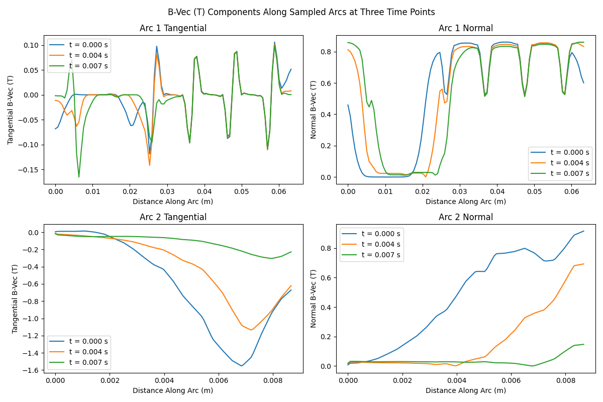
Plot tangential and normal B-Vec components
from pyemsi import Plotter, examples
from matplotlib import pyplot
import numpy as np

file_path = examples.ipm_motor_path()
plt = Plotter(file_path)

data = plt.sample_arcs(
    arcs=[
        ((0.080575, 0, 0), (0.0569751, 0.0569751, 0), (0, 0, 0)),
        ((0.0792007, 0.0167379, 0), (0.0769587, 0.0251049, 0), (0, 0, 0)),
    ],
    resolution=100,
)

fig, axes = pyplot.subplots(len(data), 2, figsize=(12, 4 * len(data)))
axes = np.array(axes, dtype=object)
if axes.ndim == 1:
    axes = axes[np.newaxis, :]

for idx, arc_data in enumerate(data):
    time_indices = sorted({0, len(arc_data) // 2, len(arc_data) - 1})

    for time_idx in time_indices:
        label = f"t = {arc_data[time_idx]['time']:.3f} s"
        axes[idx, 0].plot(
            arc_data[time_idx]["B-Vec (T)"]["distance"],
            arc_data[time_idx]["B-Vec (T)"]["tangential"],
            label=label,
        )
        axes[idx, 1].plot(
            arc_data[time_idx]["B-Vec (T)"]["distance"],
            arc_data[time_idx]["B-Vec (T)"]["normal"],
            label=label,
        )

    axes[idx, 0].set_xlabel("Distance Along Arc (m)")
    axes[idx, 0].set_ylabel("Tangential B-Vec (T)")
    axes[idx, 0].set_title(f"Arc {idx + 1} Tangential")
    axes[idx, 0].legend()

    axes[idx, 1].set_xlabel("Distance Along Arc (m)")
    axes[idx, 1].set_ylabel("Normal B-Vec (T)")
    axes[idx, 1].set_title(f"Arc {idx + 1} Normal")
    axes[idx, 1].legend()

fig.suptitle("B-Vec (T) Components Along Sampled Arcs at Three Time Points")
fig.tight_layout()
fig.savefig("docs/static/demos/sample_arcs_bvec_components_time_slices.png")
See Also
sample_arc()— Sample along a single circular arcsample_lines()— Sample along multiple straight linessample_points()— Sample at multiple point coordinates